Expert routing is flatter than you think
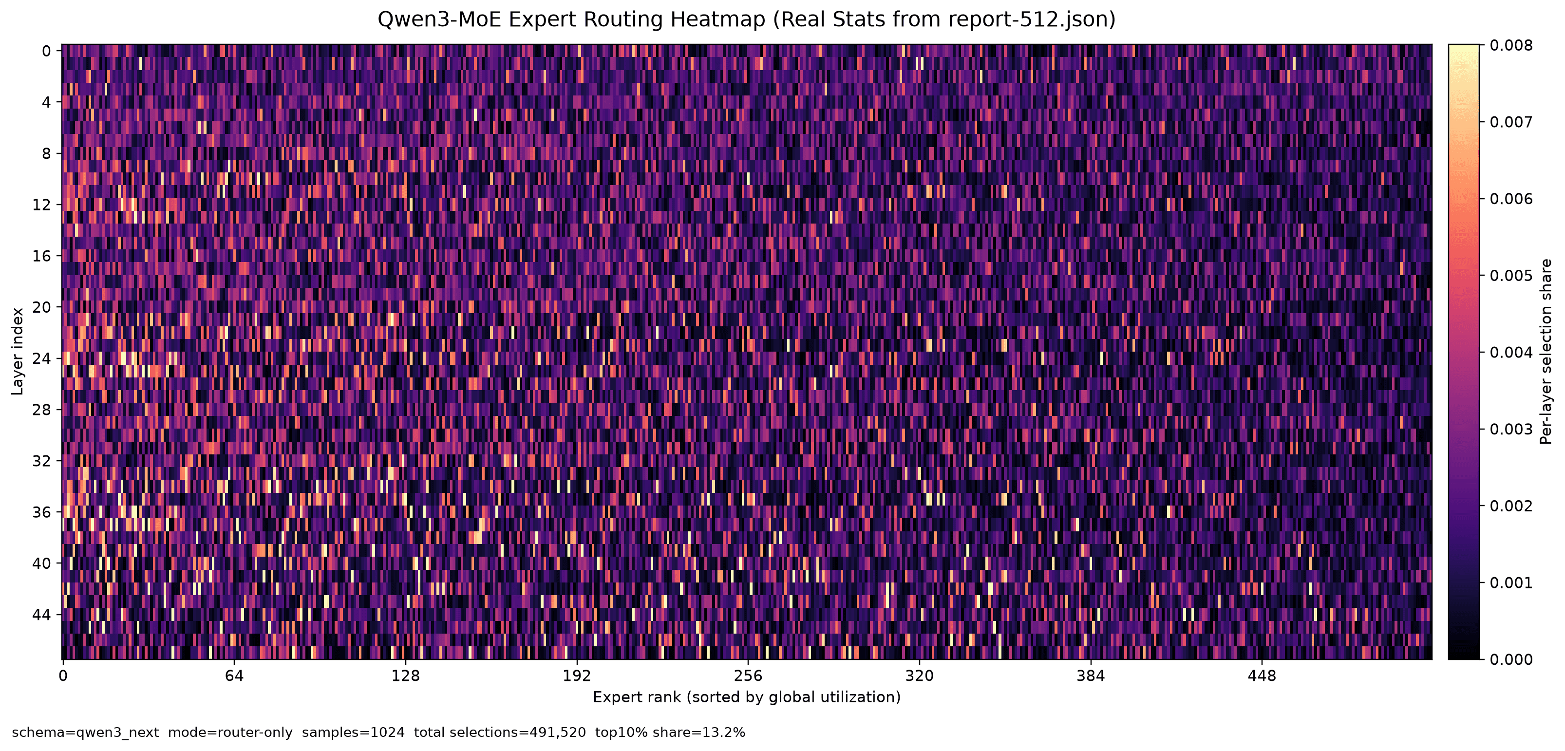
Profiling all 48 layers of Qwen3-Coder-Next gives a routing Gini of 0.1006. Almost nothing is dead, almost nothing dominates — which changes what pruning a Mixture-of-Experts checkpoint can and cannot buy you.
The folk model of a Mixture-of-Experts layer is that it degenerates. You train 512 experts, a few dozen win, the rest sit cold, and pruning is a matter of deleting the dead weight. It is a satisfying story and it makes compression sound easy.
It did not survive contact with the measurements. Profiling all 48 MoE layers of Qwen3-Coder-Next with router-only probes produced a routing Gini coefficient of 0.1006 — much closer to uniform than to collapsed. The busiest expert in the model was selected 1,453 times across 491,520 router selections; the quietest was selected 488 times. A factor of three between the extremes of 512 experts is not a winner-take-all distribution.
What the concentration curve says
The clearest way to read the distribution is to ask what share of routing mass the busiest experts take, and compare it against what uniform routing would give them.
| Bucket | Observed share | Uniform | Ratio |
|---|---|---|---|
| Top 1% | 1.42% | 1% | 1.42× |
| Top 5% | 7.02% | 5% | 1.40× |
| Top 10% | 13.22% | 10% | 1.32× |
| Top 20% | 25.04% | 20% | 1.25× |
| Top 50% | 57.12% | 50% | 1.14× |
Routing mass by expert percentile, Qwen3-Coder-Next, 48 layers, 1,024 samples. The third column is the ratio to uniform.
Every bucket is above uniform, so there is real preference in the router — but the largest ratio anywhere in the model is 1.42×. Compare that against the mental model where the top 10% of experts carry most of the forward pass. That model would put the top-10% share somewhere north of 60%. The measured value is 13.22%.
Cold experts are rare and unevenly placed
If experts are not concentrated, are any of them actually unused? Barely. Across 48 layers the mean number of cold experts per layer was 3.396 out of 512 — about 0.66%. But the distribution of that scarcity is itself uneven: 45 of the 48 layers had at least one cold expert, and one layer had 27.
That asymmetry is the practical argument for per-layer pruning over a single global ranking. A global keep-list applies one model-wide opinion about which experts matter to a layer that may disagree. The per-layer strategy ranks within each layer and keeps that layer's own winners.
So what does pruning actually buy?
Cutting 512 experts down to 128 — a 4× reduction — retained 99.34% of observed routing mass. That number is better than the flat distribution would suggest, and the reason is that top-k routing is being reduced alongside the expert count, from k=10 to k=4. You are not only removing experts; you are also asking the router to commit harder to the ones that remain.
The honest framing is this: because routing is close to uniform, pruning is not free salvage of dead capacity. It is a real trade, and coverage is the number that tells you how much you traded. A run that reports 99.34% coverage has left 0.66% of observed routing mass unserved, and those tokens now route somewhere else.
Flat routing means pruning is a decision about acceptable loss, not a free lunch. Coverage is how you price it.
Reproducing this
Router-only mode loads just the router weight tensors — a few megabytes — and probes each router with random unit-norm hidden states. The full 48-layer sweep took 4.98 seconds on CPU. No GPU, no model load.
python3 moe_monitor.py router-only \
  --model-dir Qwen/Qwen3-Coder-Next-FP8 \
  --output ./stats/report-512.json \
  --keep-experts 128 \
  --new-topk 4 \
  --samples 1024 \
  --strategy per-layer
The caveat worth stating plainly: random probes measure the router's structural preferences, not what your traffic does. A workload concentrated on one domain will produce a very different picture. That is what full-model mode and the traffic daemon are for — and the gap between the two is itself worth measuring.